Breadth First Search

Breadth first search is a core algorithm used to traverse trees that can be generalized to traversing graphs as well.

Breadth first search might remind you of level-order traversal in a tree, and is also very similar to how graph traversal was done in CPSC 110. The idea is to visit all nodes from a certain distance of the current node by putting them in a queue before marking nodes as visited and iterating over the queue.

Implementation

An example of the BFS algorithm for an adjacency list implemented graph could be something like the following (note that this requires the omitted implementation of an adjacency list graph, a node with parent and value pointers, and a state variable):

typedef enum = {EXPLORED, NEW} STATE;
 
Node* BFS(Graph g, Node* root, int targetValue){
	Queue q;
	root->state = STATE.EXPLORED;
	q.enque(root);
	
	while(!q.isEmpty()){
		Node* n = q.dequeue();
		if(n->value == targetValue){
			return n;
		}
		
		for(Node* adjNode : g.getAdjacentNodes(n)){ //for each adjacent node
			if(adjNode->state != EXPLORED){
				adjNode->state = EXPLORED;
				adjNode->parent = n;
				q.enqueue(adjNode);
			}
		}	
	}
}

Class Example

The example given in class is similar, but works with edges and I found it a little bit more complicated to wrap my head around.

Algorithm BFS(G, V)
	Input: graph G and start vertex v
	Output: labeling of edges in V's connected component as "discovery" or "cross" edges.
Queue q;
SetLabel(v, VISITED)
q.enqueue(v);
while !q.IsEmpty
	q.dequeue(v)
	for all w in G.AdjacentVertices(v)
		if(GetLabel(w) == UNVISITED)
			SetLabel(v, w, DISCOVERY)
			SetLabel(w, VISITED)
			q.enqueue(w)
		else if (GetLabel(v, w) == UNEXPLORED)
			SetLabel(v, w, CROSS)

The idea is relatively simple, we take an arbitrary starting point in a graph (or in the tree’s case, the root) and we queue each adjacent node to the current one into a FIFO queue. We then dequeue nodes from that queue until its empty. Each time we visit a node, we mark it as visited so it doesn’t accidentally get visited multiple times and create a cycle. And that’s pretty much it.

This guarantees visiting every node in a tree or a connected graph, and is relatively easy to implement.

Tip

Much like a lot of algorithms in CPSC 221, you’re not necessarily expected to know how to implement the algorithm off the top of the dome. But you are expected to know how it works and to be able to predict how BFS will act on an example graph.

Edge Types

When using BFS, because we need a way to avoid cycles, the general method is to label nodes or edges as visited to avoid requeuing them to the BFS worklist. This can work with nodes or edges interchangeably and there really isn’t that much of a difference. In this class however, we generally do so with edges and it’s pretty common to be asked what kind of edge you will end up with as a result of a BFS algorithm. BFS results in two edge types.

Discovery

Pretty self explanatory, if the edge connects the current node with an unexplored node, it is a discovery edge, an edge that has been ‘discovered’ to be part of the spanning graph.

Cross

A cross edge is basically the name given to any edge that isn’t a discovery edge. The idea is that it ‘crosses’ from one discovery path to another, and doesn’t contribute to discovering new nodes.

Example

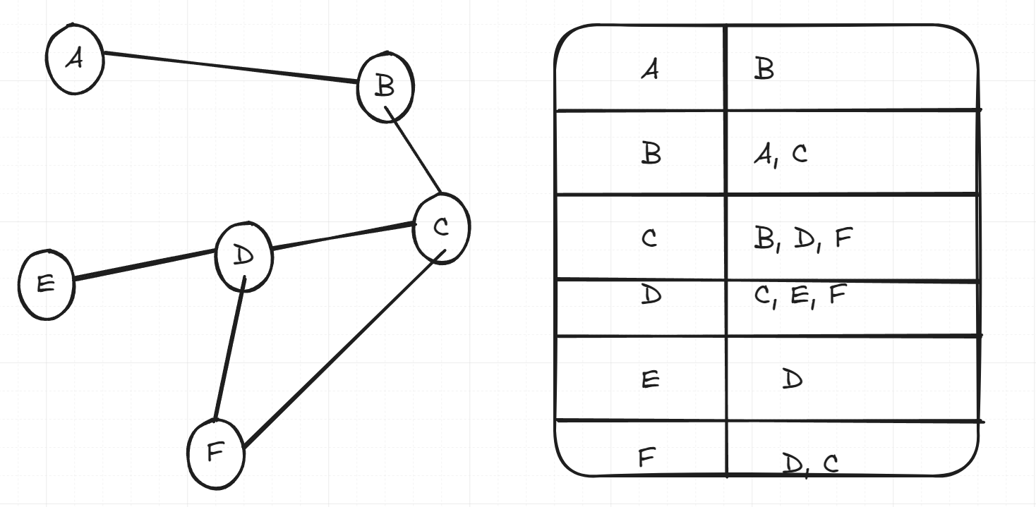
For example, see if you can trace the BFS algorithm on the following graph represented by an adjacency list, starting at the vertex A.

Answer

The order of visited nodes will of course start with A. The BFS algorithm will then queue B, who we visit next. B will then queue A, but that’s already visited so we ignore it, then C. C is at the top of the queue now, so that’s what we visit. We check B, it’s already been visited so we ignore it, we queue D and F. So now our queue contains D and F. We deque D, queue E, F has already been queue and marked as visited so we ignore it. Next on our queue is F, we visit it and don’t find any new nodes. We then visit E, who doesn’t have any new nodes. So the final order of visits would be: A B C D F E

Traversal time Complexity

Let $n$ be the number of nodes and $m$ be the number of edges.

When the breadth first search is ran on a graph represented by an adjacency list, the time complexity is:

$$O(n+m)$$

Explanation

Looking at the above example of a graph implemented with the adjacency list for example, we can see that we iterated over every node in the graph. And for every node in the graph, we iterated over its list of adjacent nodes, in other words the degree of that node, in other words we’ll also visit every edge in the graph. Therefore, our time complexity is dictated by both $n$ and $m$, and the larger of the two depends on how connected the graph is.

Note that if the graph is represented by an adjacency matrix, then the time complexity of the traversal is

$$O(n^2)$$

instead.

Explanation

In the case of an adjacency matrix, because it is represented by a 2D array, and it semantically does not record what nodes are adjacent to each other, we have to traverse each list of vertices twice to figure out whether they are adjacent or not and therefore whether we should add them to the queue or not.

Applications

Tree Detection

When running BFS, you can determine that a graph is a tree if it has no cross edges, all vertices have one parent, and all the vertices are in one connected graph.

Finding a Spanning Tree

If using an edge-based implementation, BFS also naturally forms a spanning tree, which you can return by either constructing a path while you’re traversing or by marking the edges with some kind of state.

Shortest Path Problem

If each time we visit a node, we record their parent (like in our implementation example), we can backtrack a target node to the node we started with, which will give us the shortest path to that node. In effect, breadth first search is a valid shortest path finding algorithm specifically for unweighted, undirected graphs.