AVL Tree

An AVL tree, named after Adelson Velsky and Landis, is a self-balancing binary search tree.

Properties

Since the AVL tree is a BST, it shares many of its properties. The main difference in between them is that the AVL tree is self-balancing. Since the AVL tree is always balanced, it has a maximum height of $O(log(n))$ where n is the number of nodes. To do so, the AVL tree is defined by a balance factor.

Balance Factor

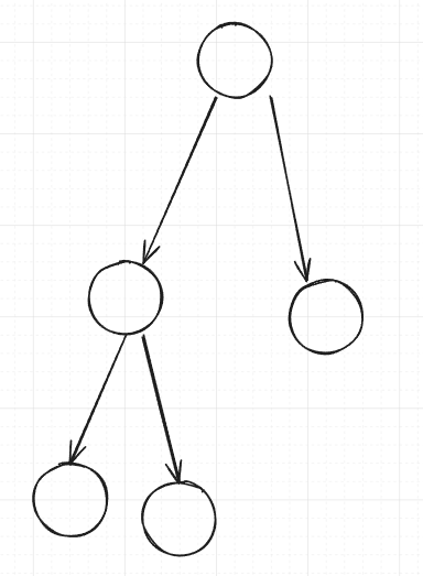
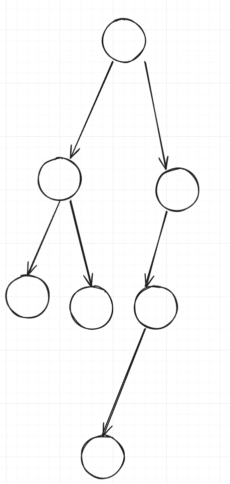
The balance factor at any node of an AVL tree is the difference in height in between its left subtree and its right subtree. A balanced tree has at most a balance factor of $|1|$ for every node in its tree. For example, try determining which of these is balanced:

Answer

This tree is balanced. The height of the left subtree of the root is 1, while the height of the right subtree of the root is 0. Therefore, the balance factor of the root is $|1|$, which is within bounds for a balanced tree. The left subtree has two children, one on each side so it has a balance factor of $0$.

Answer

This tree is not balanced. The height of the left subtree of the root is 1, while the height of the right subtree of the root is 2. Therefore, the balance factor of the root is $|1|$, which is within bounds for a balanced tree. However, the right subtree’s left side is of height 1, while its right side’s height is -1 (it’s empty), therefore a balance factor of $|2|$, which makes the tree as a whole unbalanced.

Implementation

One of the possible implementations for a node of such a tree could be something like this:

enum balance_type{ LEFT_HEAVY = -1, BALANCED = 0, RIGHT_HEAVY = 1};
 
class AVLNode {
	public: 
		int data;
		int height;
		AVLNode* left;
		AVLNode* right;
		balance_type balance;
}

Where it effectively just has extra fields that denote the balance of that node’s subtree and its height. It would also include rotations, which are they key operations that keep the AVL tree balanced.

Rotations

Balancing of the tree occurs via operations called rotations. Assuming we take the above implementation example, how would we implement rotations so that our tree self-balances correctly? To rebalance an AVL tree, we must have an algorithm that handles all types of imbalances. There are four different types of imbalance, each with their own algorithm to rebalance the tree or subtree.

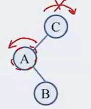
LEFT LEFT

Left left imbalance is when the source of imbalance is the subtree’s left child’s left child. It looks like this:

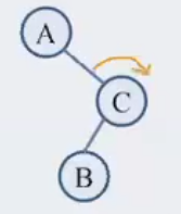
And is solved by a right rotation at C. What would do you think the resulting tree should look like?

Answer

The resulting tree looks like this:

This can be implemented with an algorithm like the following:

Node* rightRotate(Node*& n) {
    Node* newSubRoot = n->left; //the new subroot is the roots left child
    n->left = newSubRoot->right;
    //if B had a right subtree, we would shift that to the original root's left child
    newSubRoot->right = n; //shift the old root to the new ones right
    n = newSubRoot;
 
    // Update heights
    n->height = max(height(n->left), height(n->right)) + 1;
    newSubRoot->height = max(height(newSubRoot->left), height(newSubRoot->right)) + 1;
 
    // New root
    return newSubRoot;
}

Visual step-by-step

If you’re struggling to see how that works, I would recommend drawing it step by step. I did it below here, but see if you can draw it for yourself and compare to my drawings.

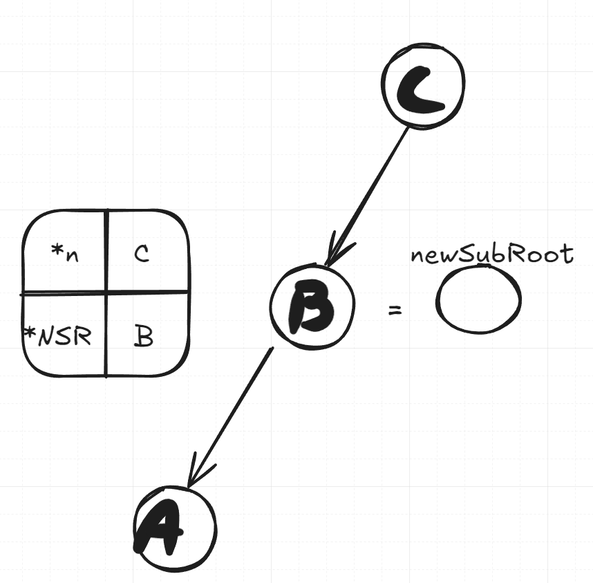
Step one

We first create a new sub root to serve as a dummy node so we don’t lose anything when we swap nodes. It’s a node pointer, and it points to the original root node’s left child, effectively being a copy of B. Keep in mind that n here in the above algorithm is the node C. We’ll keep track of what n and newSubRoot are pointing to as well at each step.

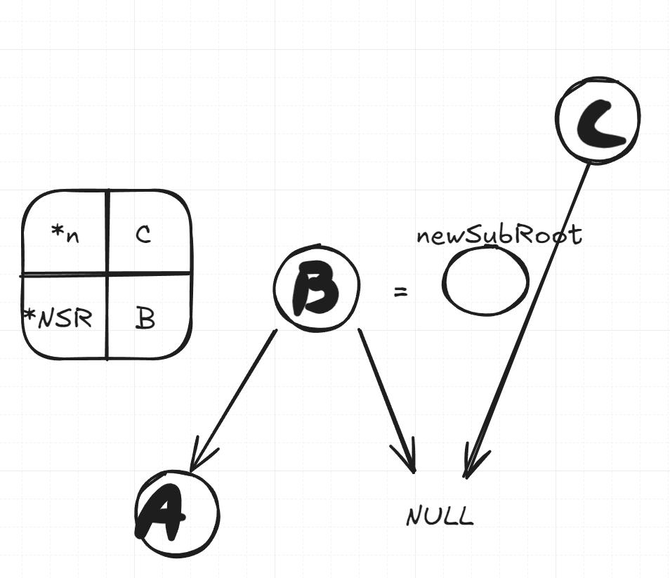
Step two

We assign C’s left node to our new subroots right node, which is equivalent to Bs right child. In this case, there is none, but if B had a right child this is where C would inherit it.

Step three

We then reassign our new sub root’s right child to be our old root. Geometrically, this is the part that actually ‘rotates’ our graph, since now the new subroot is at the top.

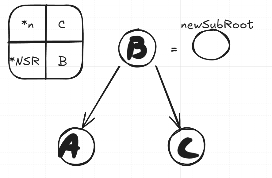
Step four

We then reassign the n pointer to point to the same node as the n pointer. In this case, n who was pointing to C now points to B. Since we pass the node pointer n by reference, this will modify the tree in place so that we don’t have to rely on the return value to reassign a root, and instead just run the function and potentially ignore the return value and it will still work.

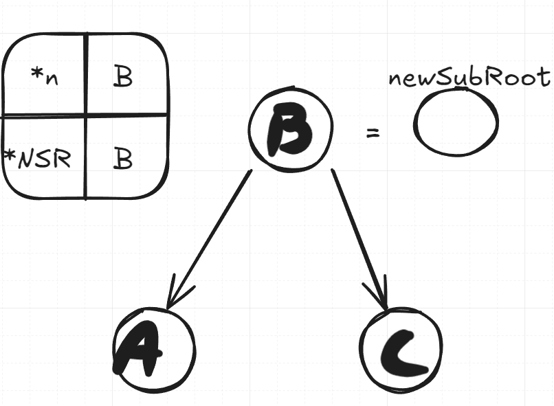
Step five

Update the tree heights and return the new sub root. Not much to draw visually here, but to note that since the new sub root and n are pointing to the same value I’m pretty sure both would be valid return values.

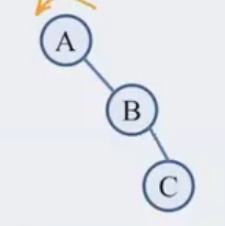
RIGHT RIGHT

Right right imbalance looks like this:

And is solved by a left rotation at A. The resulting tree looks the same as the previous one. The algorithm is effectively the same but with the left/right nodes swapped.

Node* leftRotate(Node*& n) {
    Node* newSubRoot = n->right; //the new subroot is the roots right child
    n->right = newSubRoot->left;
    //if B had a left subtree, we would shift that to the original root's (As) right child
    newSubRoot->left = n; //shift the old root to the new ones right
    n = newSubRoot;
 
    // Update heights
    n->height = max(height(n->right), height(n->left)) + 1;
    newSubRoot->height = max(height(newSubRoot->right), height(newSubRoot->left)) + 1;
 
    // New root
    return newSubRoot;
}

LEFT RIGHT

Left-right imbalance is when the source of imbalance is the subtree’s left child’s right child.

It is solved by a left rotation at A, then a right rotation at C. Note that after the left rotation at A, we effectively get the LEFT LEFT case above.

RIGHT LEFT

This imbalance is solved by a right rotation at C, then a left rotation at A. Note that after the right rotation at C, we effectively get the RIGHT RIGHT case above.

Tip

It’s pretty likely you won’t have to memorize the exact algorithm for rotations or implementations of an AVL tree. However, you do need to understand how it works and how to trace AVL insertions.

Insertion

One of the most effective ways of ensuring AVL balance is to never let it become unbalanced upon insertion in the first place.

Insertion starts with a regular BST insertion, followed by rotations to maintain balance. In other words, we maintain the properties of an AVL tree after each insertion.

Code example

An example of a code implementation of an insertion function could look something like this:

void insert(Node*& root, int key, int value){
	if(root == null){
		root = new Node(key, value);
	} else if(key < subtree->key){
		insert(subtree->left, key, value);
	} else {
		insert(subtree->right, key, value);
	}
	rebalance(subtree);
}

Effectively a generic BST insertion function with a call to a helper rebalancing function at the end of every recursive call, so when the calls start to unwind upwards, we check at every level of the tree whether it is unbalanced or not. I can’t give the exact code for the rebalancing function since it’s part of one of the labs of CPSC 221, however from the context of this article you can probably tell that the pseudo code should be something like this:

void rebalance(Node*& root){
	if(balanceFactor < -1){ //left imbalance
		if(left_left imbalance){ //how could we determine this?
			rotateRight(root);
		} else {
			 rotateLeftRight(root);
		}
	}
	//Can you tell what the other case is?
}

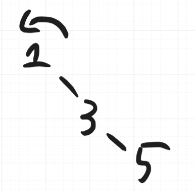
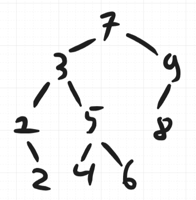
One of the best ways to check your own understanding on this topic is to see if you can predict what an AVL tree would look like after a certain number of random insertions. Try your hand at predicting what an AVL tree that was initially empty would look like after insertions of 1, 3, 5, 7, 9, 8, 6, 4, 2.

Answer

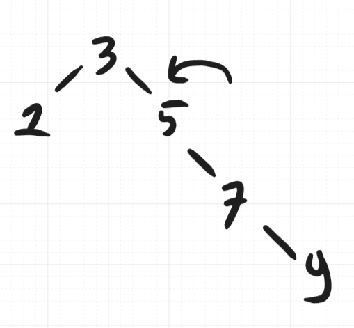
We insert following a standard BST algorithm and at every point we’ll check if any nodes are unbalanced. Our first unbalanced situation is this one:

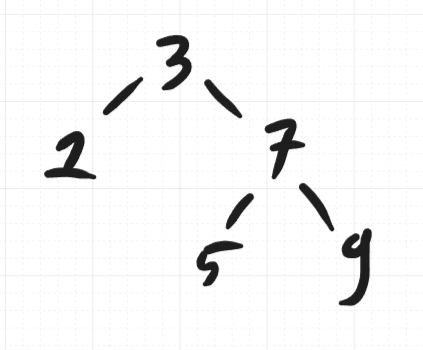
Where after three insertions we have exactly the RIGHT RIGHT imbalance mentioned earlier in the article. So, we rotate left on the root, which is 1. We then keep inserting until we hit another imbalanced case, where we have yet another RIGHT RIGHT imbalance. We do another left rotation, this time on the root’s right child:

Which results in the following structure:

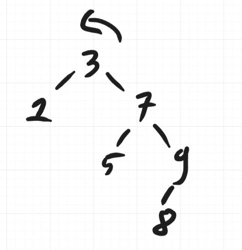
We then keep inserting until we get to our final imbalanced case for this sequence of insertions, where we can once again notice a RIGHT RIGHT imbalance.

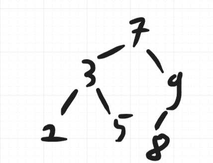
We perform another left rotation on the root, which results in the following:

Note how 3 inherited 7’s left child. Then we keep inserting and we don’t encounter any imbalanced cases, and we end up with the following tree:

Did you get the same result?

Common Problems

One common type of problem you’re likely to encounter is how to transform a degenerate binary tree (in this class they also sometimes call it a spine or a stick) into a proper AVL tree. Try to figure this one out for yourself.